Generative Art January
On the seldom chance that I come across it and have free time, I’ve been inspired by generative art that uses functions, code, and principles of data visualization to create beautiful things. I also find it a great way to practice fundamentals of coding.
Here are my very few contributions to “Genuary”, and code to replicate them.
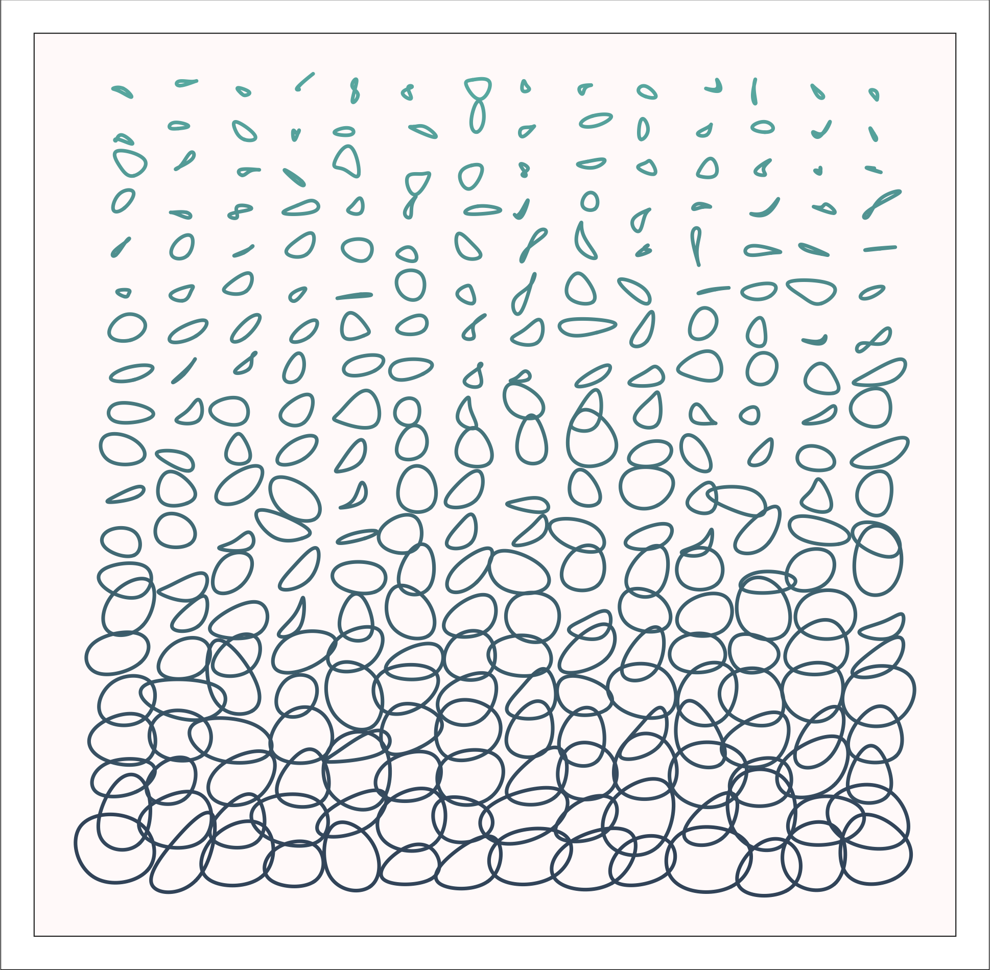
Prompt: Increase the randomness across the Y-axis (pictured above)
Here, I used groups of four points, each arranged around central coordinates across a y-axis, and added a nudge in a random direction to each of the four points, with the nudge increasing with the central y-coordinate. I then used BSplines around each group of four to create “circles” around the invisible anchor points, creating the effect pictured above. Then I slapped on a color gradient, just for fun.
See the code!
#-----------------------------------------------------------------------------
library(tidyverse)
library(ggforce)

n <- 20 # set number of circles
cols <- 14 # set number of columns

plot <-
  # make base grid
  data.frame(group=1:(n*cols),
                   basex=rep(c(1:cols),each=n)*4,
                   basey= (1:n)) %>%
  # generate randomness
  mutate(
    x = lapply(basey/2, function(x)
    {y = rnorm(4, basey, basey)
    x*c(-1, 1, 1, -1) + y}),
    y = lapply(basey/2, function(x)
    {y = rnorm(4, basey, basey)
    x*c(1, 1, -1, -1) + y})
  )  %>%
  unnest(cols = c(x,y)) %>%
  # add randomness to base grid and expand
  mutate(newy = y + basey*10.5,
         newx = x + basex*3.8) %>%
  # plot
  ggplot(aes(x=newx,y=newy,color=(newy),group=group,fill=(newy))) +
  geom_bspline_closed(show.legend = F,alpha=.7,size=.8,fill=NA) +
  coord_equal(expand = T)+
  theme_void()+
  # flip plot
  scale_y_reverse()+
  scale_color_gradient(high="#40556b",low="#67b5af")+
  theme(panel.background  = element_rect(color="grey20",fill="snow",size=.5),
        plot.background = element_rect(color="black",size=.3),
        plot.margin = margin(.55,.55,.55,.55,"cm"))

ggsave(plot, filename = here::here("R Projects","genuary19_3.55.png"),dpi=300)
#-----------------------------------------------------------------------------
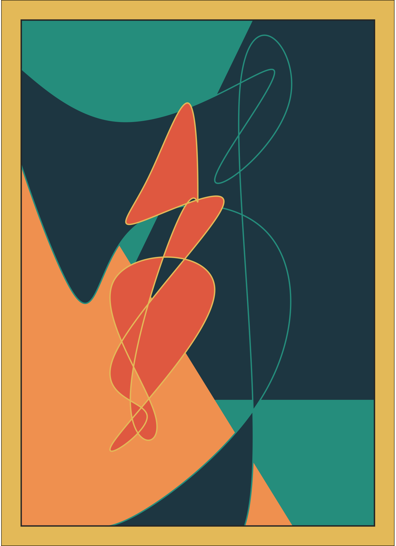
Prompt: Do anything with these 5 colors
Woah - no limits! Here, I developed two styles of randomly generated designs that change with each run (as new random numbers are selected).
First, a modern-art-inspired piece using some geom_ribbons with random slopes behind two groups of randomly generated data points fitted with geom_bspline_closed functions creating curved objects, with fill colors randomly selected for each object out of the five.
See the code!
#-----------------------------------------------------------------------------
library(tidyverse)
library(ggforce)

# set some parameters
pal <- c("#264653", "#2a9d8f", "#e9c46a", "#f4a261", "#e76f51")
nrow <- 10
ncol <- 7
npoints <- 13

# create and print plot
{set.seed(1)
  p <- ggplot()+
    # add a triangle
    geom_ribbon(aes(y=c(0:(ncol+1)),
                    ymin=sample(10,1),
                    ymax=(runif(1,0,3)*c(0:(ncol+1))),
                    x=c(0:(ncol+1))),
                fill=pal[sample(1:5,1)])+
    # and another
    geom_ribbon(aes(y=c(0:(ncol+1)),
                    ymin=-5,
                    ymax=(runif(1,-2,-1)*c(0:(ncol+1))+nrow),
                    x=c(0:(ncol+1))),
                fill=pal[sample(1:5,1)]) +
    # add curved shapes
    geom_bspline_closed(aes(x = sample((0-2):(ncol+2), npoints, replace = T),
                            y = sample( (0-2):(nrow+2), npoints, replace = T)),
                        fill=pal[sample(1:5,1)],
                        color=pal[sample(1:5,1)],
                        n=1000) +
    geom_bspline_closed(aes(x = sample(1:(ncol-1), npoints, replace = T),
                            y = sample( nrow, npoints, replace = T)),
                        fill=pal[sample(1:5,1)],
                        color=pal[sample(1:5,1)],
                        n=1000) +

    # add a frame
    geom_rect(aes(xmin=0.5,
                  xmax=ncol+.5,
                  ymin=0.5,
                  ymax=nrow+.5),
              color="grey20",
              fill=NA,
              size=1)+

    scale_fill_manual(values=pal) +
    scale_color_manual(values=pal) +
    theme_void() +
    theme(panel.background = element_rect(color="grey20", fill=pal[sample(1:5,1)],
                                          #fill="white",
                                          size=1
    ),
    legend.position = "none",
    plot.background = element_rect(color="black",size=.3,fill=pal[sample(1:5,1)]),
    plot.margin = margin(.55,.55,.55,.55,"cm"))+

    coord_equal(xlim = c(0.5,ncol+.5),
                ylim = c(0.5,nrow+.5),
                expand = F)
  print(p)

  # remove the pound signs below to save the plot
  #ggsave(filename = here::here("p.png"),
  #       width = 4.6,
  #       height = 6.1,
  #       dpi=300)
}
#-----------------------------------------------------------------------------
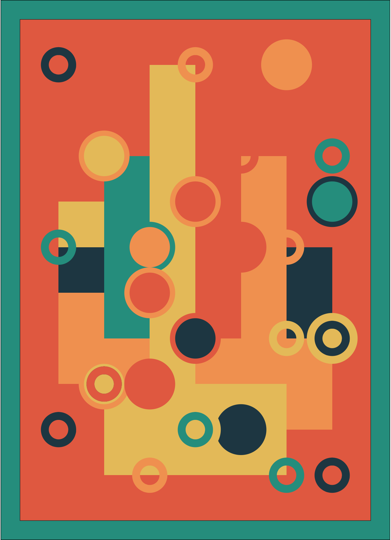
Second, a geometric collection of geoms using coordinates randomly sampled from a 7x10 coordinate plane.
See the code!
#-----------------------------------------------------------------------------
library(tidyverse)

# create some parameters
nrow <- 10
ncol <- 7
pal <- c("#264653", "#2a9d8f", "#e9c46a", "#f4a261", "#e76f51")
nsquares <- 25
ncircles <- 12
ncircles2 <- 15
radius=.5

# make plot
#----------------------------------------------------
{set.seed(7) # change seed number for different random data
  plot <- ggplot() +

    # add random squares
    geom_rect(aes(xmin=sample(ncol, nsquares, replace = T),
                  xmax = sample(ncol, nsquares, replace = T),
                  ymin=sample( nrow, nsquares, replace = T),
                  ymax=sample( nrow, nsquares, replace = T),
                  fill=sample(pal, nsquares, replace=T))) +

    # add random circles
    geom_circle(aes(x0=sample(ncol, ncircles, replace = T),
                    y0=sample(nrow, ncircles, replace = T),
                    r = radius,
                    fill= sample(pal, ncircles, replace=T),
                    color=sample(pal, ncircles, replace=T)),
                size=2) +


    # add smaller random circles
    geom_circle(data =  data.frame(x = sample(ncol, ncircles2, replace = T),
                                   y = sample( nrow, ncircles2, replace = T),
                                   color = sample(pal, ncircles2, replace=T)),
                aes(x0=x,y0=y,r=(radius-.2),color=color),fill="transparent",size=3) +

    coord_equal(xlim = c(0.5,ncol+.5),
                ylim = c(0.5,nrow+.5))+

    scale_fill_manual(values=pal) +
    scale_color_manual(values=pal) +
    theme_void() +
    theme(panel.background = element_rect(color="grey20", fill=pal[sample(1:5,1)]),
          legend.position = "none",
          plot.background = element_rect(color="black",size=.3,fill=pal[sample(1:5,1)]),
          plot.margin = margin(.55,.55,.55,.55,"cm"))
  print(plot)
  #ggsave(filename =here::here("plot.png"),
  #       width = 4.6,
  #       height = 6.1,
  #       dpi=300)
}
#-----------------------------------------------------------------------------